Graphs, their traversal and use cases – I

Hi!
In High School we have already studied graphs and how they are used to showcase our data but in Computer Science, Graphs as a Data Structure are a completely different concept. We use graphs to represent relationships between one or more entities. The nodes represent the entities and relationships are depicted by edges. A graph G is represented as (V, E) in which V is the set of vertices and E is the set of edges. Today, we’ll be exploring it out further.

What you can see above is a simple undirected graph depicting the friendship(relationship) using edges between various people(nodes). What we can concur from the above graph is that Krishna is Divij’s and Ramesh’s friend, while Krishna’s friends are both Divij and Ramesh. What you might have noticed is I used the term undirected, and that should strike your curiosity that how many other types of graphs are possible?
The answer to that question is:

• Undirected and Directed
• Weighted and Unweighted
• Simple and Non-simple
• Sparse and Dense
• Cyclic and Acyclic
• Embedded and Topological
• Implicit and Explicit
• Labelled and Unlabeled

I know I have listed a lot but we’ll not be going through each and every graph type in detail. We’ll only cover undirected, directed, weighted, unweighted, cyclic and acyclic graphs.

• Undirected vs Directed: The edges of directed graph will imply the receiver and sender for the specified relationship, whereas in undirected graph both nodes act as receiver and sender.
• Weighted vs Unweighted: The edges of weighted graph not only depict the relationship but also the strength of the relationship, and in various cases, the cost of the relationship. The unweighted graph only depicts the relationship.
• Cyclic vs Acyclic: As the names might suggest, cyclic graph contains a cycle, whereas acyclic graphs do not.

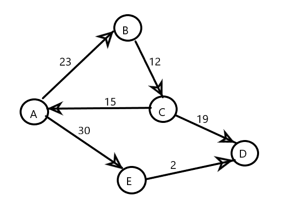
Above you can see the two graphs representing the road network between various cities(A, B, C, D and E) with edges depicting the cost of toll on each road.
In the first graph if you start from A, you will eventually end up on D but the cost you pay will depend on your decisions on which path to choose. Later on in this blog we will discuss an algorithm to find the path with minimal cost.
Now, take a look at the second graph in which we have a cycle between nodes A, B and C. The cost will increase each time you re-enter the cycle and might occur infinitely depending on your code. Later on we will take a look at how to find these cycles in a graph.

After all this theory I hope the coder in you is still eager to open up your fav text editor and ready to encounter some errors! Before we move on to coding, I would like to explain one last thing which is how to represent Graphs in your code. There are two ways to represent graphs:

• Adjacency Matrix
• Adjacency List

For a graph G = (V,E) with n and m elements in V and E respectively, adjacency matrix will be a nxn matrix with each cell containing the weight of the edge connecting the two vertices.
On the other hand, adjacency list contains a linked list corresponding to the vertex and shows the various vertices it is connected to.

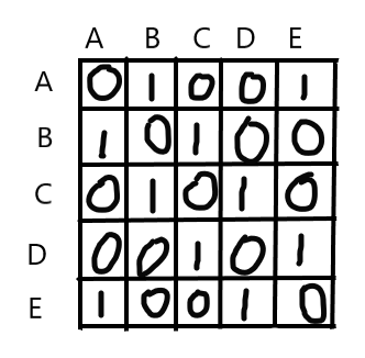
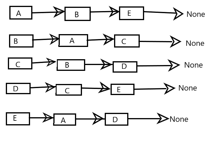
Let’s see if you grasp the concept or not. For the undirected and unweighted graph above, try to write the adjacency matrix and the adjacency list. Take your time!
Following is the answer:

I have given you the solution to unweighted graphs but now try to make the Adjacency Matrix and Adjacency List for the weighted graph specified above. If you have any problems or doubts, feel free to reach out to me via comments or email me.

Let’s get our hands dirty with some code! As you might already know, every code will be in Python.

from collections import defaultdict #defaultdict is used for initializing the dictionary with empty list 

class Graph:
    def __init__(self, N):
        self.N = N
        self.graph = defaultdict(list)

    def addEdge(self, v, u):
        self.graph[v].append(u) # Node v is connected to node u
        self.graph[u].append(v) # Node u is connected to node v

g1 = Graph(5) 
g1.addEdge(1, 0) 
g1.addEdge(0, 2) 
g1.addEdge(0, 3) 
g1.addEdge(3, 4)

print(g1.graph) 
"""

Output:
defaultdict(<class 'list'>, 
{1: [0], 
0: [1, 2, 3], 
2: [0],
3: [0, 4],
4: [3]})
"""

The above python program incorporates the Adjacency List approach to representing Graphs. If you notice, the program will only show connected graphs. If there are nodes which are not connected to any node, they will not be considered. Now I will show you the representation using Adjacency Matrix.

class Graph:
    def __init__(self, N):
        self.N = N
        self.graph = [[0]*N for _ in range(N)] #initializing the matrix with 0s to specify that no nodes are yet connected

    def addEdge(self, v, u):
        self.graph[u][v] = 1 # Edge from u to v exists
        self.graph[v][u] = 1 # Edge from v to u exists
    
g1 = Graph(5) 
g1.addEdge(1, 0) 
g1.addEdge(0, 2) 
g1.addEdge(0, 3) 
g1.addEdge(3, 4)

print(g1.graph)
"""

Output:
[[0, 1, 1, 1, 0], 
[1, 0, 0, 0, 0],
[1, 0, 0, 0, 0],
[1, 0, 0, 0, 1],
[0, 0, 0, 1, 0]]
"""

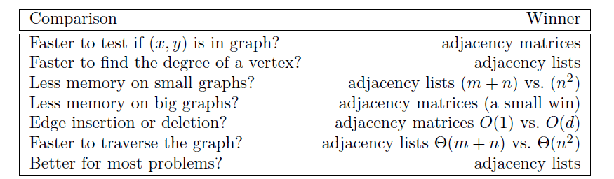
In this approach every node is taken into consideration which makes the complexity of traversal θ(n^2) whereas the complexity of traversal in Adjacency List is θ(m+n).
For a more detailed comparison you can take a look at The Algorithm Design Manual by Steven S Skiena but for the crux of it:

In the next session, we’ll take a look at various algorithms used for traversing graphs and how they are used for solving problems.